Category Archives: Excel Tips and Tricks

Essential Excel Shortcuts to Master Your Table Data

Note: Click on the video above to watch.

Show Off In Meetings with these Excel Tips!

Navigating and showcasing data in Excel can be a breeze with the right shortcuts. Whether you’re presenting data to your boss or analyzing large datasets, these handy tips will streamline your workflow and make your reports stand out. Let’s dive into some essential Excel shortcuts to enhance your data management skills.

1. Select Entire Table

To quickly select all your data in a table, use:

  • Ctrl + A, or
  • Ctrl + Shift + Spacebar

These shortcuts highlight your entire table, making it easy to apply formatting or make bulk changes.

2. Convert Data to Table

Turning your data into a formal table can help with organization and filtering. Simply press:

  • Ctrl + T

This converts your selected range into a table, allowing for easier manipulation and formatting.

3. Add Filters

To add filters to your data, which is crucial for sorting and analyzing information, use:

  • Ctrl + Shift + L

This will add filter dropdowns to your table headers, making it simple to filter and view specific data subsets.

4. Insert a Slicer

For a more visual way to filter data, especially useful in presentations, you can add a slicer:

  • Select a cell in your table.
  • Go to the Table Design tab and click Insert Slicer.
  • Choose the fields you want to filter by, such as “Job Title”.

Slicers make it easy to filter and display data in a way that’s clear and interactive.

5. AutoSum

To quickly calculate the sum of a column or row, select the empty cell where you want the total to appear and press:

  • Alt + =

Excel will automatically sum up the numbers above or to the left of the selected cell.

6. Find Top and Bottom Values

To find the top or bottom values in a dataset:

  • Use =LARGE(range, n) to find the nth largest value.
  • Use =SMALL(range, n) to find the nth smallest value.

For example, to find the top 3 salaries, use =LARGE(range, 1), =LARGE(range, 2), and =LARGE(range, 3).

7. Trace Formulas

To troubleshoot or verify formulas while you’re in a meeting, you can instantly go to where the formula gets its data from:

  • Press Ctrl + [ to jump to the cells referenced by a formula.
  • Press Ctrl + ] to see which cells are dependent on the selected formula.

You can also view all formulas in your worksheet by pressing:

  • Ctrl + `

This shows all formulas in your spreadsheet, helping you audit your data.

8. Trace Formulas with Arrows

To visually trace the relationships between formulas:

  • Go to Formulas > Trace Precedents or use the shortcut Alt, T, U, T to add arrows showing which cells affect the formula.

This is a great way to identify and correct any errors in your formulas.

9. Create a Pivot Table

For advanced data analysis, create a pivot table by pressing: Alt, N, V, T

This opens the PivotTable creation dialog, letting you summarize and analyze your data efficiently.

Conclusion

Mastering these Excel shortcuts will not only save you time but also help you present your data in a professional and effective manner. Whether you’re preparing for a meeting or just organizing your data, these tips will ensure you navigate and showcase your tables with ease. Happy Excel-ing!

See more Excel Tips and Tricks articles: 

You can see what people are saying about David McLachlan here: REVIEWS

Navigate to Free Project Management and Leadership Articles through the links on the right (or at the bottom if on Mobile) 

PMI PMP 35 PDUs CourseThe Ultimate PMP Project Management Prep Course (35 PDUs)
Agile Certified Practitioner (PMI-ACP 21 PDUs)The Complete Agile Course: PMI-ACP (21 PDUs), Coaching, Jira and MORE! 
50 Project Management Templates Gantt Chart Risk Matrix and more Excel50+ Project Management Templates in Excel and PowerPoint (Gantt Chart, Risk Matrix and more!)
Project Management Plan TemplatesPre-made Project Management Plan Template: Save 100 HOURS!


20 Excel Shortcuts to Clean Up Your Spreadsheet Like a Pro

Note: Click on the video above to watch.

20 Excel Formatting Shortcuts to Clean up Your Data

If you’ve ever copied data into an Excel spreadsheet only for it to come out as a jumbled mess, you know how frustrating it can be to get everything looking just right. The good news is, here are over 20 formatting shortcuts that will help you tidy up your data and get it ready to impress your boss in no time. Let’s transform your chaotic columns into a perfectly formatted spreadsheet!

1. Select All Cells in a Column

To quickly select all cells below your current cell, press Ctrl Shift ↓.

To quickly select the entire table, use Ctrl A. To select all cells in a column or row, use Ctrl Space for columns and Shift Space for rows. This grabs every cell in that column or row, making it easier to apply changes.

2. General Number Format

Got a bunch of numbers and you want to set them to general format? Use Ctrl Shift ~ (that’s the tilde key next to the number 1) to revert them to a general number format.

3. Date Format

To format a column of dates consistently, select the column and press Ctrl Shift # (the hash key). This will give your dates a standard format.

4. Time Format

For times that are all over the place, select the column and press Ctrl Shift @ to apply a uniform time format.

5. Currency Format

To give your numbers a currency makeover, select the cells and press Ctrl Shift $. This will add dollar signs and standardize the formatting.

6. Scientific Format

If you need scientific notation, select your numbers and press Ctrl Shift ^. Perfect for those large or small numbers.

7. Percentage Format

Turn your numbers into percentages by selecting the cells and pressing Ctrl Shift %. If you need more decimal places, use Alt, H, 0 (zero) to add them. Press Alt, H, 9 to reduce decimals.

8. Remove Dollar Signs

If you want to get rid of dollar signs and revert to just numbers, select the cells and press Ctrl Shift ! (the exclamation mark key).

9. Select a Range of Cells

Use Ctrl Shift combined with the arrow keys (left, right, up, or down) to select a range of cells in the direction you choose.

10. Open Formatting Dialog

For more detailed formatting options, hold Ctrl and press 1. This opens the format cells dialog box where you can adjust everything manually.

11. Add Cells

To insert new cells, select where you want to add them and press Ctrl Shift + D. This allows you to expand your table with additional cells.

12. Remove Cells

To delete cells, use Ctrl – (minus sign). This will let you remove cells from your table quickly.

13. Copy and Paste Cells

Copy your selected cells with Ctrl C, and paste them with Ctrl V.

14. Bold Text

Make your text stand out by selecting it and pressing Ctrl B to bold it.

15. Italicize Text

For a bit of emphasis, use Ctrl I to italicize your selected text.

16. Underline Text

To underline text, select it and press Ctrl U.

17. Strikethrough Text

If you need to show text as strikethrough, use Ctrl 5. This crosses out your text for clear visibility.

18. Undo Changes

Made a mistake? Press Ctrl Z to undo your last action. It’s your safety net.

19. Redo Changes

Changed your mind again? Use Ctrl Y to redo the last undone action.

20. Resize Rows or Columns

To adjust the size of rows or columns, select them and use your mouse to drag the borders, or use the shortcut Alt, H, O, I to auto-fit the columns.

There you have it – more than 20 shortcuts to make formatting your spreadsheet a breeze. Whether you’re tidying up data or making it look sharp, these shortcuts will save you time and frustration. So go ahead, give them a try and watch your data transform from messy to immaculate in an instant!

Catch you next time with more handy tips and tricks. Happy formatting!

See more Excel Tips and Tricks: 

You can see what people are saying about David McLachlan here: REVIEWS

Navigate to Free Project Management and Leadership Articles through the links on the right (or at the bottom if on Mobile) 

PMI PMP 35 PDUs CourseThe Ultimate PMP Project Management Prep Course (35 PDUs)
Agile Certified Practitioner (PMI-ACP 21 PDUs)The Complete Agile Course: PMI-ACP (21 PDUs), Coaching, Jira and MORE! 
50 Project Management Templates Gantt Chart Risk Matrix and more Excel50+ Project Management Templates in Excel and PowerPoint (Gantt Chart, Risk Matrix and more!)
Project Management Plan TemplatesPre-made Project Management Plan Template: Save 100 HOURS!


9 Excel Features you MUST know – 15 Minute Zero to Hero

comic boy learning at computerExcel is a powerful tool that can enhance your productivity in project management, data analysis, and many other fields.

What if you want to become a superhero in Excel in just 15 minutes? This video and article show you the 9 tips you need to be amazing in Microsoft Excel, and your boss and colleagues will truly be amazed! Here they are – the nine essential Excel features that you should know to amaze your friends:

1. Pivot Tables

Pivot tables are a great way to summarize large sets of data. They allow you to organize and manipulate your data to get a simplified view.

To create a pivot table:

  • Select your data range and format it as a table.
  • Go to Insert > PivotTable.
  • Choose the data range and decide where you want the pivot table to be placed.
  • Drag and drop fields to rows, columns, values, and filters sections to customize your pivot table.

For example, you can count the number of job titles in different countries and filter the data by departments.

2. VLOOKUP

VLOOKUP is used to find and retrieve data from a specific column in a table.

To use VLOOKUP:

  • Type =VLOOKUP(lookup_value, table array or area, column number you’re looking for, Exact Match yes or no).

For example, =VLOOKUP(A2, data_table, 2, FALSE) will search for the value in cell A2 within “table array or area” and return the corresponding value from the second (2) column. This is particularly useful when you need to match employee IDs with their names, job titles, salaries, and bonuses.

3. Quick Analysis and Data Bars

Quick Analysis allows you to apply conditional formatting, create charts, and more with a few clicks.

To use Quick Analysis:

  • Select your data range.
  • Click the Quick Analysis button that appears at the bottom right.
  • Choose options like Data Bars, Color Scale, or Icon Set to visualize your data quickly.

Data bars visually represent the value in each cell, making it easy to see variations at a glance.

4. IF Then Else Statements

IF statements help you perform logical tests and return different values based on the results.

To create an IF statement:

  • Type =IF(logical_test, value_if_true, value_if_false).

For example, =IF(B2 > 100000, “Yes”, “No”) will check if the value in B2 is greater than 100,000 and return “Yes” or “No” accordingly.

This can be used to check if salaries exceed a certain amount.

5. Spark Lines

Spark lines are tiny charts within a cell that provide a visual representation of data trends.

To insert spark lines:

  • Select your data range.
  • Go to Insert > Sparkline > Line.
  • Choose the data range and the cell where you want the sparkline to appear.

Spark lines are useful for displaying trends in salaries across different countries.

6. Wildcard

Wildcards allow you to perform partial matches in your data searches.

To use a wildcard:

  • Type =COUNTIF(range, “*criteria*”).

For example, =COUNTIF(B2:B10, “*manager*”) will count the number of cells that contain the word “manager” within the specified range.

This feature helps in searching for specific terms within job titles.

7. TRIM

TRIM removes unwanted spaces from text.

To use TRIM:

  • Type =TRIM(text).
  • For example, =TRIM(A2) will remove any extra spaces from the text in cell A2.

This ensures that your data is clean and free of unnecessary spaces.

8. Transpose

Transpose changes the orientation of your data from rows to columns or vice versa.

To transpose data:

  • Select your data range and copy it.
  • Right-click where you want to paste the data, choose Paste Special, and select Transpose.

This feature is useful for reorganizing data to fit your needs.

9. Case Conversion

Excel functions can change text to uppercase, lowercase, or proper case.

To change case:

  • Use =UPPER(text) to convert to uppercase.
  • Use =LOWER(text) to convert to lowercase.
  • Use =PROPER(text) to convert to proper case.
  • For example, =UPPER(A2) will change the text in A2 to all uppercase letters.

These nine features can significantly enhance your efficiency and effectiveness in using Excel. Practice these techniques to get up to speed with Excel quickly and make your data management tasks easier and more productive. Happy Excelling!

See more Excel Tips and Tricks: 

You can see what people are saying about David McLachlan here: REVIEWS

Navigate to Free Project Management and Leadership Articles through the links on the right (or at the bottom if on Mobile) 
PMI PMP 35 PDUs CourseThe Ultimate PMP Project Management Prep Course (35 PDUs)
Agile Certified Practitioner (PMI-ACP 21 PDUs)The Complete Agile Course: PMI-ACP (21 PDUs), Coaching, Jira and MORE! 
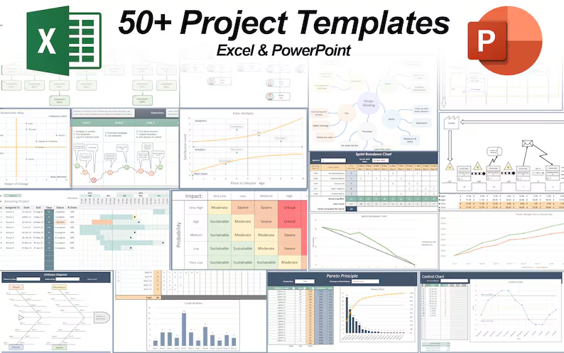
50 Project Management Templates Gantt Chart Risk Matrix and more Excel50+ Project Management Templates in Excel and PowerPoint (Gantt Chart, Risk Matrix and more!)
Project Management Plan TemplatesPre-made Project Management Plan Template: Save 100 HOURS!


How to Count Colored Cells in Excel (3 Ways)

Excel doesn’t have a formula to count colored cells, so here are three fantastic, easy ways to count colored cells in Excel.

Way 1: Using a Filter

  1. Select the range of colors with the header cell included
  2. Go to Home > Sort & Filter > Add Filter
  3. Click on the down-arrow in the header cell, Sort by Color, and select the color you want.

Now you can count the sorted cells and see how many of that color there are.

Way 2: Using Name Manager

This way is more powerful, faster, but a bit more complicated.

  1. Select the cell NEXT TO the range you want to count color in (in this picture it’s C3)
  2. Go to Formulas > Name Manager > New Name
  3. Input the new name (something like ColorCount, but it’s your choice)
  4. Input the formula: =GET.CELL(38, B3)
    • (“38” checks the cell color attribute)
  5. Now in the cell next to your colored column, input your new formula: “=ColorCount” and drag it down the column. It will give you the “Numbers” that associate with the colors in the cell next to it.
  6. Now in a separate cell with the color you want to count next to it (E and F columns in the picture), input “=COUNTIF(E3, ColorCount)”
    • Where E3 is the color you want to count, and ColorCount is our Named formula from before.

This will count ALL the colors that match that color!

Way 3: Creating a Formula to Count Color Using VBA

The final, coolest, fastest and most automatic way is to create our very own Formula in Excel that does exactly what we need. We’ll do this using VBA, and you can see how easy it is to create your own formulas!

  1. Select Developer > Visual Basic
  2. In the VBA Window, Select Insert > Module
  3. In the Module window that appears, input the below VBA code, then close the window (it saves automatically).
  4. Finally, use your new formula in any cell: =COUNTINGCOLORS( Range of Colors, Cell with the color you want to count)

The code is:

Function COUNTINGCOLORS(MYRANGE As RANGE, MYCOLOR As RANGE)

Dim COLORCELL As Integer
Dim CURRENTCOUNT As Integer

COLORCELL = MYCOLOR.Interior.ColorIndex

Set CELL = MYRANGE

For Each CELL In MYRANGE
If CELL.Interior.ColorIndex = COLORCELL Then
CURRENTCOUNT = CURRENTCOUNT + 1
End If

Next CELL
COUNTINGCOLORS = CURRENTCOUNT

End Function

See more Excel Tips and Tricks: 

You can see what people are saying about David McLachlan here: REVIEWS

Navigate to Free Project Management and Leadership Articles through the links on the right (or at the bottom if on Mobile) 

PMI PMP 35 PDUs CourseThe Ultimate PMP Project Management Prep Course (35 PDUs)
Agile Certified Practitioner (PMI-ACP 21 PDUs)The Complete Agile Course: PMI-ACP (21 PDUs), Coaching, Jira and MORE! 
50 Project Management Templates Gantt Chart Risk Matrix and more Excel50+ Project Management Templates in Excel and PowerPoint (Gantt Chart, Risk Matrix and more!)
Project Management Plan TemplatesPre-made Project Management Plan Template: Save 100 HOURS!